


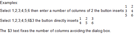
Math-Science is a Microsoft Word Add-in programmed as a Word template in Visual Basic for Application.
Math-Science add new tabs to Microsoft Word ribbon:
Math tab:

The Math tab offers tools to format math expression using the new Word Math Expression editor since Word 2007, to draw geometric drawings, 3D objets, and many others.
Functions tab:

The Functions tab offers tools to to draw functions curves, variation and signs tables, tables of values, statistics and conics.
Physics tab:


The Physics tab offers an oscilloscope screen tool with 4 inputs, an optical banc tool to draw rays across a converging or diverging lens.
Each group give access to a library of drawing in electricity, mechanics, optics, acoustics.
Chemistry tab:


The Chemistry tab offers shortcuts to insert ions, acid-base couples, redox couples, atoms of the first 2 lines of the Mendeleev classification, radioactive elements.
Tools inserts acid-base titration, and conductometric titrations, acid-base predominance diagrams, and advancement tables of a chemical reaction.
A library of drawings gives access to the glassware in 2D and 3D, as well as to common apparatus and equipment, and to symbols of danger.
A Chemical Formula Editor draws basic developed and semi-developed chemical formula's.
Scidot tab:

The Scidot tab gives access to the template Options, to the Help file, to a Handbook of Physics and Chemistry constants.
You can configure the template to display only the tabs you want, and in each tab the groups you want to display.
A scroll down list allows to change the template language.
The Activation button display the activation status and allows you to enter your activation key.
License:
Math-Science requires a license for permanent use. 28 days of free trial period.
Installation:
Run the Math-Science.exe executable file.
Enter the MS activation key included in the invoice email.
For a test try, do not enter any activation key, and you will enter a 28 days trial period.
At any time, you will find the latest version of the Math-Science template on our web site http://scidot.com.
How to activate the template to your Microsoft Word documents ?
With the default installation parameter, the Math-Science template is not loaded with Microsoft Word, but only is a small template in the Add-Ins tabs that has one button to load/unload the template to your current Microsoft Word document. To load the Math-Science template when Microsoft Word starts, check the box in the installation dialog box.
When Microsoft Word starts, if the Add-Ins tab is missing, or if the Math-Science tabs are missing, please read on our website http://scidot.com at the Frequently Asked Question page under the paragraph 4, how to solve this problem that is due to a Microsoft Word program interruption.
Contact:
SCIDOT
24 rue Madeleine Brès
75013 PARIS
France
email: mail@scidot.com
web: http://scidot.com
phone: +33.145.886.143
Math tab
The Equation Editor group:
EQ Not selected: grey : formatting expressions are done with Word Equation Editor.
Selected: yellow or blue: formatting expressions are done with the font defined in the Options and using fields codes.
{a} Display/Hide fields codes.
The Math Expressions group:
-
+
+
The following tools use Microsoft Equation Editor. In the Math-Science option, you can ask to switch to the previous formatting mode using field codes.
Shortcut Ctrl+Maj+M.
Example.
Shortcut Ctrl+Maj+A.
Shortcut Ctrl+Maj+V.
Shortcut Ctrl+Maj+F.
Example : 3,x to write the cubic root of x.
Shortcut Ctrl+Maj+R.
Shortcut Ctrl+Maj+E.
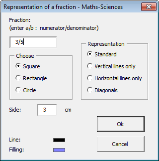
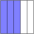
Building figures example.
Example.
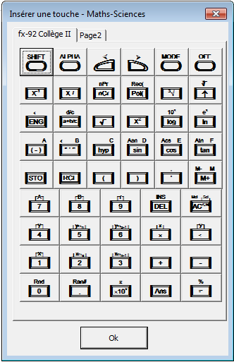
When no text is selected, a dialog box opens to insert the fx-92 calculator keys.. Example.
Example: When you select 3+4.5 the result "= 7.5" is inserted after the selection.
+
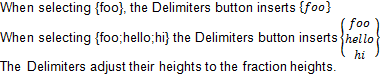
This menu allows you to write delimiters around an expression with brackets, square brackets, rounded brackets, and with a bar or a double bar.
The delimiter can be drawn on the right, on the left or on both sides.
A list of expression separated by commas will be displayed within the selected delimiter.
To avoid that the command understand a comma as a new expression, you have to enter \ (backslash) before it.
Example.
-
Insert an operation as done with the pencil. Insert a calculation tree. Convert units.
.
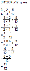
Fractions are simplified and set to the greatest common denominator.
Example.
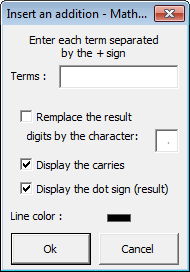
When no addition is selected: displays the addition dialog box.
When an addition is selected: inserts the addition without options.
Example.
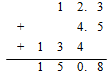
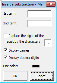
When no addition is selected: displays the substraction dialog box.
When an addition is selected: inserts the substraction without options.
Example.
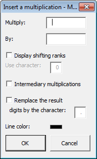
When no addition is selected: displays the multiplication dialog box.
When an addition is selected: inserts the multiplication without options
Example.
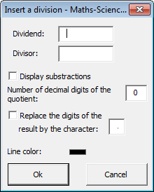
When no addition is selected: displays the division dialog box.
When an addition is selected: inserts the division without options
Example.
Usefull to compute simple conversions between units.
Example: When you select 3,4m=cm the button inserts 3,4m= 340 cm
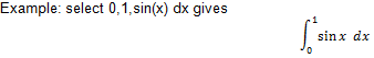
Enter a function. Compute the value at a given point. Derivate a function. Compose two functions.
Example.
+
The College group :
Without selection a dialog box is displayed to enter the 3 elements. Select the 3 elements separated by a comma a,b,expr, insert the sum.
Example.
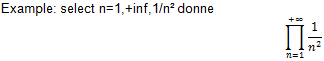
Without selection a dialog box is displayed to enter the 3 elements. Select the 3 elements separated by a comma a,b,expr, insert the product.
Example.
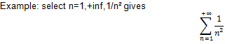
Without selection a dialog box is displayed to enter the 3 elements. Select the 3 elements separated by a comma a,b,f(x)dx, insert the integral sum.
Shortcut Ctrl+Maj+I.
Example.
Without selection a dialog box is displayed to enter the 2 elements. Select the 2 elements separated by a comma a,b, insert the arrangement.
Example.
Without selection a dialog box is displayed to enter the 2 elements. Select the 2 elements separated by a comma a,b, insert the combinaison.
Example.
Without selection a dialog box is displayed to enter the 2 elements. Select the 2 elements separated by a comma a,b, insert the combinaison with parenthesis.
Example.
Without selection a dialog box is displayed to enter the 3 elements. Select the 3 elements separated by a comma a,b,f(x)dx, insert the primitive form.
Example.
Without selection a dialog box is displayed to enter the 3 elements. Select the 3 elements separated by a comma x,0,f(x), insert the limit.
Shortcut Ctrl+Maj+L.
Example.
For first and second derivatives and differentials.
Example.
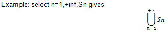
Without selection a dialog box is displayed to enter the 3 elements. When selecting an element, this one is placed next to the union symbol.
Example.
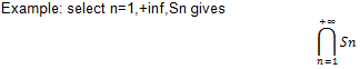
Without selection a dialog box is displayed to enter the 3 elements. When selecting an element, this one is placed next to the intersection symbol.
Example.
Without selection a dialog box is displayed to enter the element to be placed under the tilde. When selecting an element, this one is placed under the tilde symbol.
Example.
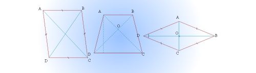
The Geometry group:

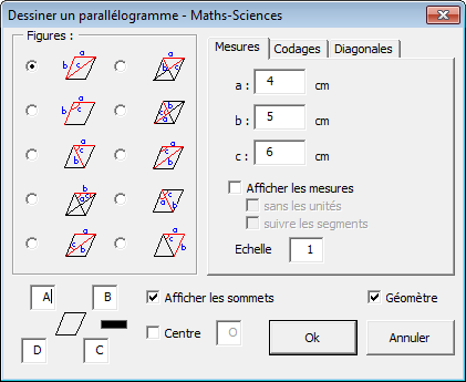
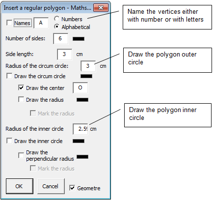
This button opens a dialog box to build a geometric drawing step by step.
Example.
-
Menu :
Example.
Example.
Example.
Sous-menu :
Example.
-
-
-
Example.
Example.
-
Example.
Example.
Example.
Example.
Example.
-
Example.
Example.
Exemple.
Example.
Sub-menu:
Example.
Example.
Example.
Example.
-
Sub-menu:
Example.
Example.
-
Example.
Example.
Example.
Example.
-
Example.
Sub-menu:
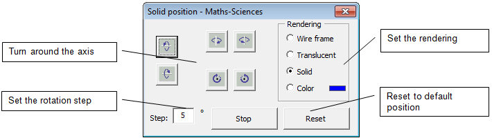
For each 3D objets, once drawn, a dialog box is diplayed to move the object around.
Example.
-
Sub-menu:
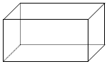
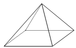
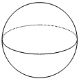
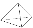
Inserts the perspectives of a cube, pavoid, cylinder or a prism.
-
Sub-menu:
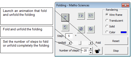
Inserts the folding of the following solids:
Example.
-
Sub-menu:
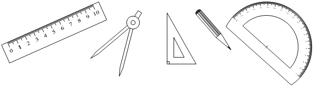
Inserts instruments used in plane geometry.
With the compass, the rule and the set-square, the selection of a line set the distance of the compass, the length of the rule, or the direction of the set-square.
Example.
+
Menu:
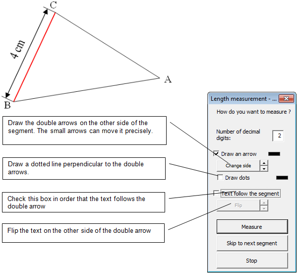
Select a polygon, and click one of these measurement: you can measure the polygon sides length, its perimeter, its angles and its area. You can also measure the length of a circle and the area of a disc.
Example.
+
If a folding is selected, you can fold and unfold it.
+
Menu
For all transformations, you must select the objects in a defined order (and this is very important): first click on the first object, then keep the Shift key pressed and click on the following objects.
Beware, since Word 2007, you cannot define an axis or a center with the 'line' tool. You must now use the 'free form' tool: first click to define the first point of the line, second click to define the second point of the line, then press the 'ESC' key to end the line.
Then enter the rotation angle in the dialog box.
Then enter the homothetie coefficient in the dialog box.
+
This button opens a dialog box to build a geometric drawing step by step.
Example.
The Symbols group:
Insert a symbol at the current cursor position.
Use the new Word 2007/2010/2013 equation editor format if applicable.
The Alignments group:
Example: After drawing a triangle, and Dissociate, you can choose a different color for every side of the triangle.
Regroup: When an element of a group is selected, this command regroup the former group it belong to.
If "Page" is selected before, all the objects are moved to get an equal horizontal distribution over the page.
If "Page" is selected before, all the objects are moved to get an equal vertical distribution over the page.
The Construction group:
To build a geometrical drawing you must operate in this order:
1. Place a Text Area that in which you will describe the geometrical drawing and whose dimension will define the geometrical drawing.
2. Insert the geometrical description by using the Group menus.
3. To avoid marks, type for the first line "No marks" en début de texte.
4. Run the geometrical drawing tracing.
Example.
Quickparts:
- Programatic Quick Insertions Ctrl+Shift+M
- Automatic Quick Insertions Ctrl+Shift+Y
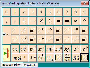
Inserts characters and maths-expressions using Word Equation Editor.
Inserts Physics and Chemistry constants.
Note: the EQ button is not functionnal with the simplified equation editor.
You can also access to this function by selecting a text expression and right click on it : a context menu is displayed with the Expression button.
Functions:
Greek letter are inserted when typed (use \ if bad interpretation).
example : 2alpha/3
The operand * is replaced by ×
The operand : or / is replaced by ÷
tex(a;b;c) inserts the text a with b in superscript and c in subscript
mes(AB) inserts an horizontal bar on the top of the selected text
ang(AB) inserts an inner angle
ren(AB) inserts an outer angle
vec(AB) inserts a vector
sqr(AB) inserts a square root
nor(AB) inserts a norm
exp(expr) inserts the exponantial function
log(expr) inserts the logarithm function
ln(expr) inserts the naeperian logarithm function
cos(expr) inserts the cosine function
abs(expr) inserts the absolute value function
bar(expr) stroke the selected text out
som(i=1;N;f(i)) inserts a sum
pro(i=1;N;f(i)) inserts a product
int(a;b;f(x).dx) inserts an integral sum
lim(x;0;f(x)) inserts a limit
sys(expr1;expr2;..;exprN) inserts a system of equations
uni(i=1;N;xi) inserts an union
ins(i=1;N;xi) inserts an intersection
arr(n;p) inserst an arrangement
com(n;p) inserts a combination
cob(n;p) inserts a combination with brackets
par(a;b) inserts brackets around a above b
par(a\;b) inserts brackets around a followed by a semi-colon and b
cro(a;b) inserts square-brackets around a above b
cro(a\;b) inserts square-brackets around a followed by a semi-colon and b
acc(a;b) inserts rounded-brackets around a above b
acc(a\;b) inserts rounded-brackets around a followed by a semi-colon and b
mat(type of delimitor;number of columns;1; 2 ; 3; 4) inserts a matrix
(0 : none ; 1: brackets ; 2 : bars ; 3 : square-brackets)
del(0;g;expr) insert a delimitor around an expression, here expr is delimited with a left bracket
(0:bracket, 1:square-bracket, 2: rounded-bracket, 3:simple bar, 4:double barre, 5:open-open square-brackets, 6:open-closed square-brackets, 7:closed-open square-brackets)
(b:both side, g:only left, d:only right)
ex: del(6;b;1;2) insert the closed-open interval 1;2
Symbols:
inf infinite
drond differential
app is part of
cont has the element
tinf much smaller than
tsup much greater than
propa proportional to
plusminus plus and minus superposed
minusplus minus and plus superposed
rond function composition
Greek letters
alpha
beta
gamma
delta
epsilon
dzeta
eta
theta
iota
kappa
lamda
mu
nu
xi
ksi
omicron
pi
rho
sigma
tau
upsilon
phi
khi
psi
omega
Combinations of functions are allowed:
f(x)=abs(x-1)+tan(x+\pi)/4
Options : see the Scidot tab/Math-Science options.
This button give access to a symbolic calculator.
Example: to compute 1/2+1/3, select:
Then click on the Calculator button, the result is displayed:
0,83333333
To obtain the result as fraction, click on the the Calculator button, then click on the fraction checkbox, then Exit the Calculator dialog box and redo the previous calculation.
Example: to define the f(x) function, select:
Then click on the Calculator button to register the expression in the symbol table.
Example: to recall the definition of f(x), select:
Then click on the Calculatrice button to recall its definition.
Example: to compute f(1), select:
Then click on the Calculator button to display the result.
2
When you do not select anything, the calculator is displayed.
To define x, enter:
x=1
When typing f(x) you will compute the value of the f function at the x-value defined previously.
You can also define a function from another function:
g(x)=1+f(x)
You can define a function as the derivate of another function.
g(x)=derive(f(x))
The when typing g(x)?? you will get developped expression of g in x:
g(x)=2x
You can request to display the symbol table by typing ?? or by clicking on the Symbols button.
When clicking on the fraction checkbox, every numeric result will be display as a fraction.
When clicking on Write Result, the result is written in the current document instead of in the calculator window.
When clicking on Erase Definitions, this will reset the Symbol Tables.
To compose function, enter for example:
h(x)=f(cos(x))
Then h(x)?? gives h(x)=(cos(x))²+1
and h(1) , like h(pi) gives 2
When clicking on Reset, the calculator windows is emptied.
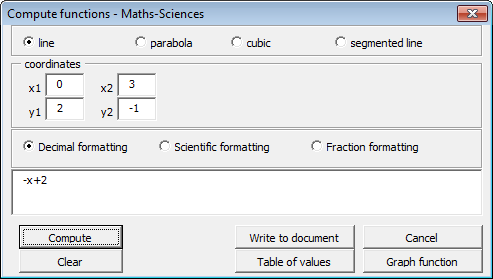
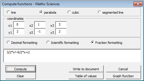
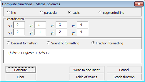
The expression generator can compute:
- the equation of a line given two points
- the equation of a parabolic curve given three points
- the equation of a cubic curve given four points
and then:
- write the expression in the current document
- launch the table of values program
- launch the graphing function program
To compute an expression, click on the Expression Generator button.
Note : the calculated coefficients are written either with the decimal, or scientific or fractionnal form.
To calculate the expression of a line, enter two points then click on Compute:
To calculate the expression of a parabolic curve, enter three points then click on Compute:
To calculate the expression of a cubic curve, enter four points then click on Compute:
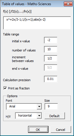
The Table of values command allows:
- to create a table of values (horizontal or vertical) for one or many function of x
- to fill a table of values. To do this, place the cursor in a Word table.
With this you can create table of values for a set of x-values you can choose.
To create a table of values, choose Table of values and enter the function of x in the dialog box displayed.
Read the math expressions rules
Enter :
the initial x value
the number of values
the increment between two values
the calculation precision
Choose if you want to Display values as fractions.
Fractions are calculated for pi, and for the square roots of 2, 3, 5 to a denominator of 12
Standard fractions are calculated to a denominator of 1000.
Note : fractions are not calculated for expressions using the exp,ln,log,10e functions.
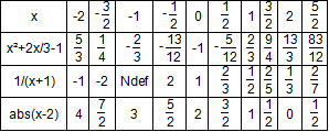
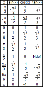
Result:
Example with fractions of pi :
Result:
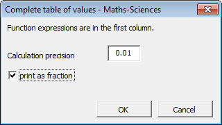
Fill a table of values :
Fill the empty cells with the computations of the expressions entered in the first line or the first column of the table.
Result:

Expressions options:
In Word equation editor mode (EQ button is grey), the equations are displayed using Word equation editor in the size specified (font is Calibria Math).
In Field code mode (EQ button is blue or yellow), the equations are displayed directly in the font and size specified (field codes are used for fractions).
Note: when a value is not defined the computer displays Ndef.
- sqr(x) when x<0
- 1/x when x=0
- ln(x) and log(x) when x<0
- tan(x) when x=pi/2+k pi
- acs(x) and asn(x) when x<-1 or x>1
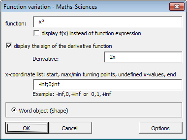
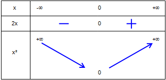
To draw a function variation table, enter
- the function expression in x
- the interval start value
- the x values of the turning points and undefined x values in the order they occur
- the interval end value
and click on the Function variation button.
Or click on the Function variation button and enter the function expression, then the list of x-values
Read the math expressions rules
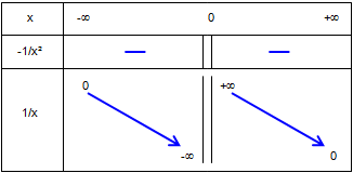
Example 1:
The function 1/x always decreases from -inf to inf :
Click on the Function variation button, the following dialog box is displayed, and enter :
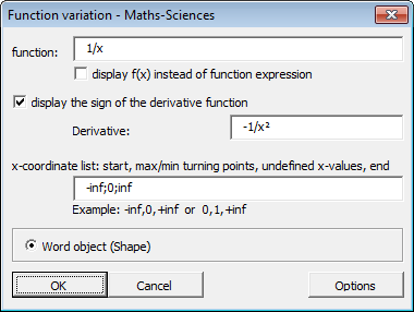
Check the table range and the list of turning points and undefined values,
and optionally change the graphical parameters, and click OK.
Example 2:
The squared function x² has x=0 as a turning point.
To draw the variation table between -inf and +inf, enter:
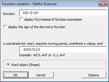
Example 3:
The function 1/(x-1) - 1/x has x= 0.5 as a turning point and is undefined when x = 0 and when x = 1.
To get the variation table between -2 and 2, enter :
Expressions options:
In Word equation editor mode (EQ button is grey), the equations are displayed using Word equation editor in the size specified (font is Calibria Math).
In Field code mode (EQ button is blue or yellow), the equations are displayed directly in the font and size specified (field codes are used for fractions).
Insert a table of variation either from a dialog box to build the table, or from another that compute it from the function expression.
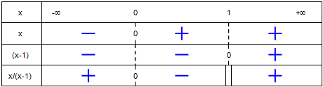
To draw a table of signs, click on the Table of signs button and enter the expressions separated by a comma and the list of x-values where the sign changes.
Example: sign of the expressions x,(x-1),x/(x-1):
Click on Table of signs, the dialog box opens:
Enter the start and end x-values and those where the sign changes, the click OK.
Expressions options:
In Word equation editor mode (EQ button is grey), the equations are displayed using Word equation editor in the size specified (font is Calibria Math).
In Field code mode (EQ button is blue or yellow), the equations are displayed directly in the font and size specified (field codes are used for fractions).
Options:
table size.
Before clicking on the Grid button, you can type a command to insert:
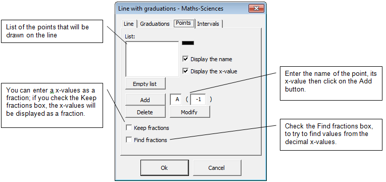
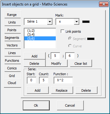
- points from their coordinates
- lines from their equations
- vectors from the coordinates of their representant
- conics like ELLIPSE, HYPERBOLA and PARABOLA
The tabs will be filled with the commands.
Examples:
To insert a grid with points:
- Type and select A(1;-2)B(-3;2.5) then click on the Grid button.
To insert a grid with vectors:
- Type and select {1;-2;-3;2.5}{2;1;0;2} then click on the Grid button.
To insert a grid with lines:
- Type and select y=x+5;x=2 then click on the Grid button.
To insert a grid with a conic:
- Type and select ELLIPSE(4;3) then click on the Grid button.
You can mix all these commands:
- Type and select A(1;-2)B(-3;2.5){1;-2;-3;2.5}{2;1;0;2}y=x+5;x=2.
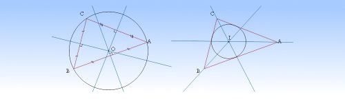
You can can:
- change the triangle sides
- give a name to each vertex
- display the sides measurements
- draw the remarkables lines
- draw the inner and outer circles
- draw points on the sides and draws parallel lines or perpendicular lines passing by the vertices.
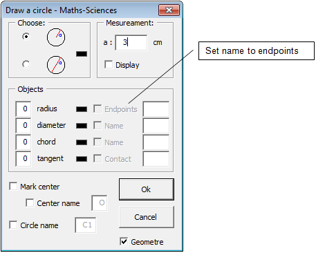
Note: if a segment is selected, a prompt will ask whether this segment will be a radius or a diameter of the circle.
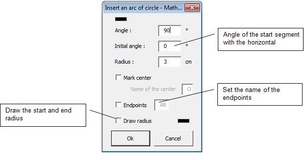
If a segment if selected, the dialog box will be filled in order to draw an arc of circle having the segment as diameter.
If a free form with 3 vertices if selected, the dialog box will be filled in order to draw an arc of circle with the the segments as radius.
and displays the following dialog box to change the parts colors:
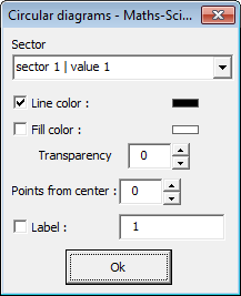
and displays the following dialog box to change the parts colors:
To enter the data, you have three choices:
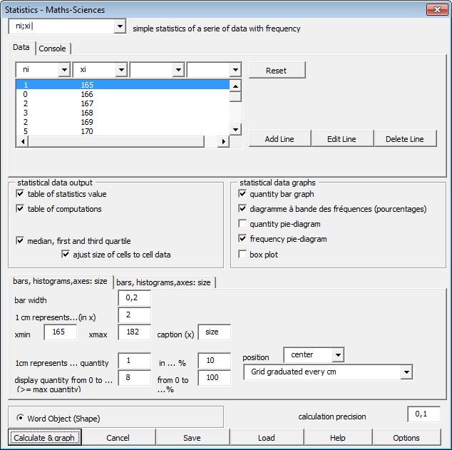
- Insert a Word table with in each line a set of data, then click on the Statistics button (cursor in the table). If the table has less than 4 rows, you will be prompted whether the set of data are in lines (default) or in columns.
- Click on the Statistics button, then enter the data with the user interface (Add button, ...).
- Enter the data in console mode. For example, for a ni,xi serie: n1;x1|n2;x2|...|nN;xN
Then from the drop down list, choose the type of statistics. This will dertermin the kind of calculations and graphics that will be executed by the Statistics module.
Statistics 1: ni; nom_classe i
Frequency (percentages) calculation:
Enter in a Word table:
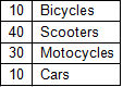
Then click on the Statistics button.
The statistics data are entered in the user interface.
(if required, add, edit or delete data)
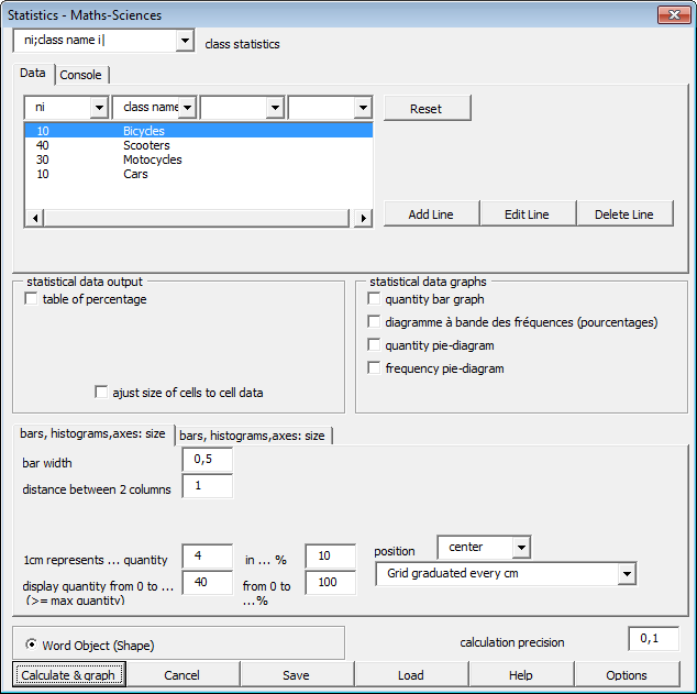
For bar graphs, you have to enter xmin and xmax (quantity), and the scale (1 cm represents...).
Frequency table (frequency are rounded so that the sum equals 100):
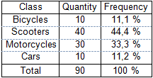
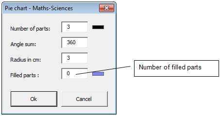
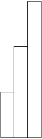
Quantity bar graph, frequency bar graph, frequency pie-diagram.
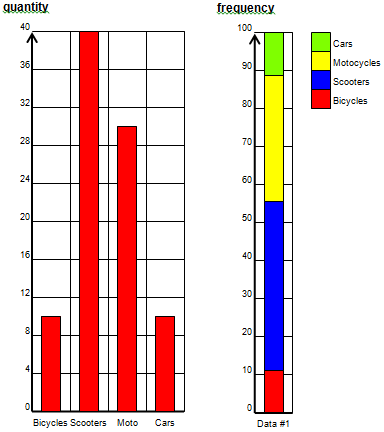
Missing image: b33-15.png
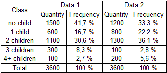
Statistics 2: ni1; ni2; class_name i
Frequency calculation of a statistics taken in two differents instants or place
Enter the data in a Word table:
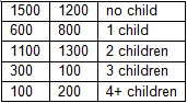
Then click on the Statistics button.
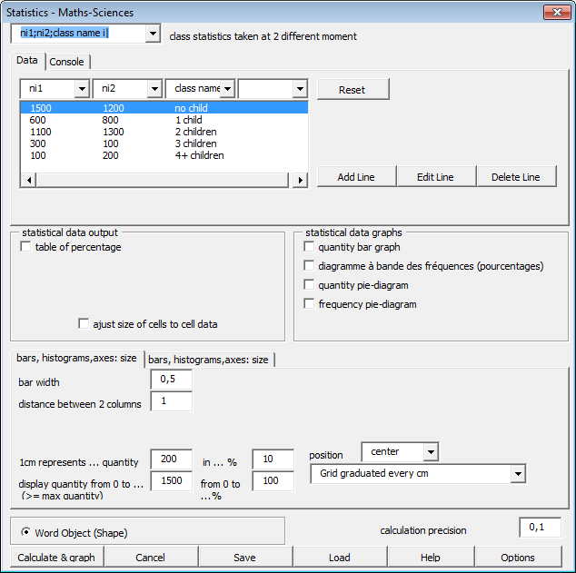
Result:
Statistics 3: xi
Statistics of a collection of data
Enter the data in a Word table:
Then click on the Statistics button:
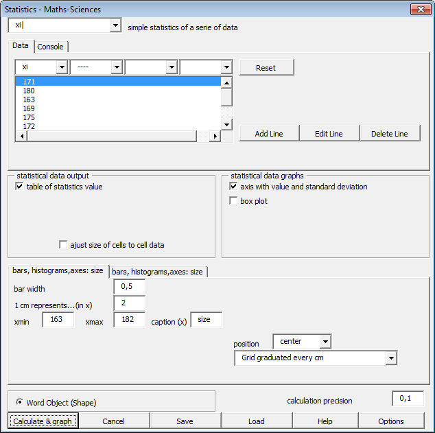
xmin=160 xmax=185 1cm represents 2.
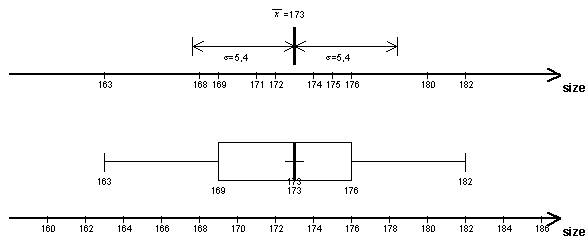
We can get the table of statistics values, the axis with the mean and standard deviation, the axis with the box plot.
In this example, the mean (cross in box plot) equals the median (large line in box plot).
The result has been done in two steps.
First the axis has been graduated with the data.
Second the axis has been graduated according to the scale.
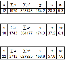
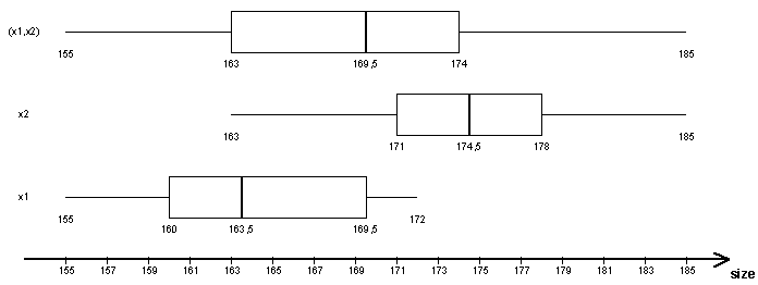
Statistics 4: xi1,xi2
Statistics of a collection of 2 data sets representing the same variable
Enter the data in a Word table:
Then click on the Statistics button:
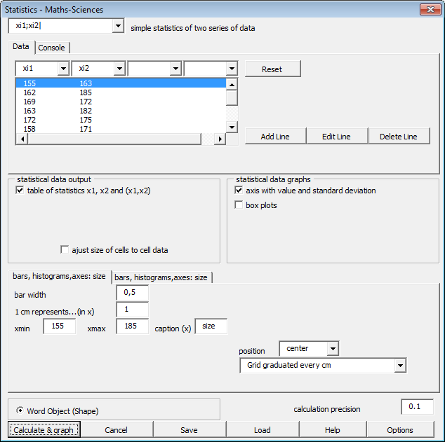
xmin=160 xmax=185 1cm represents 2.
We can get the table of table of statistics values in x1, in x2 and in (x1,x2) ; the axis with the mean and the standard deviation of x1, of x2 and of (x1,x2), so for the box plot.
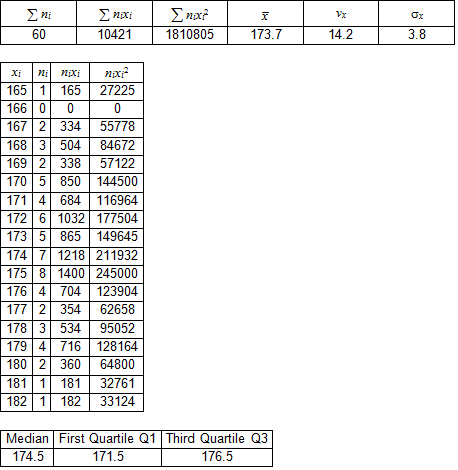
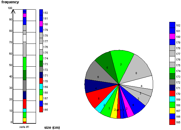
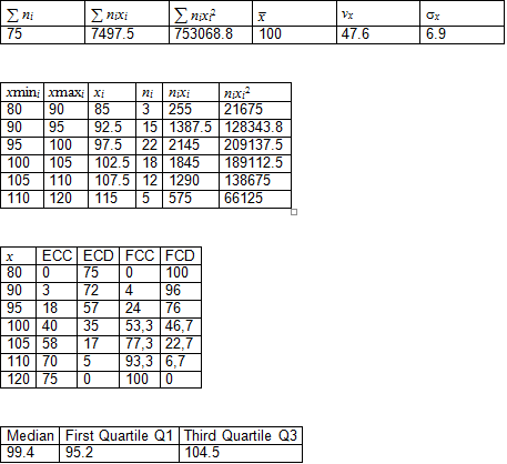
Statistics 5: ni,xi
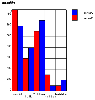
Statistics of a collection of data (quantity, class variable)
Enter the data in a Word table:
Then click on the Statistics button:
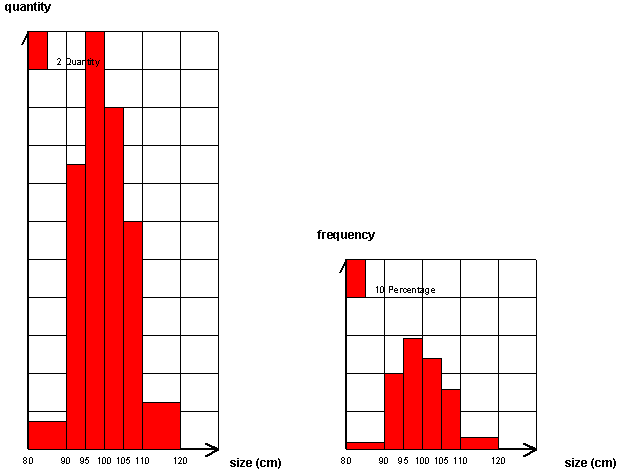
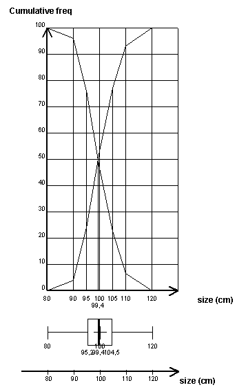
We can get the table of the statistics, the quantity bar graph, the frequency bar graph, the frequency pie-diagram, the axis with the box plot.
Statistics 6: ni,xmin,xmaxi
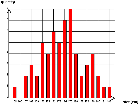
Statistics of continuous data : histograms
Enter the data in a Word table:
Here : number of child of this size, size min, size max
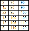
Then click on the Statistics button:
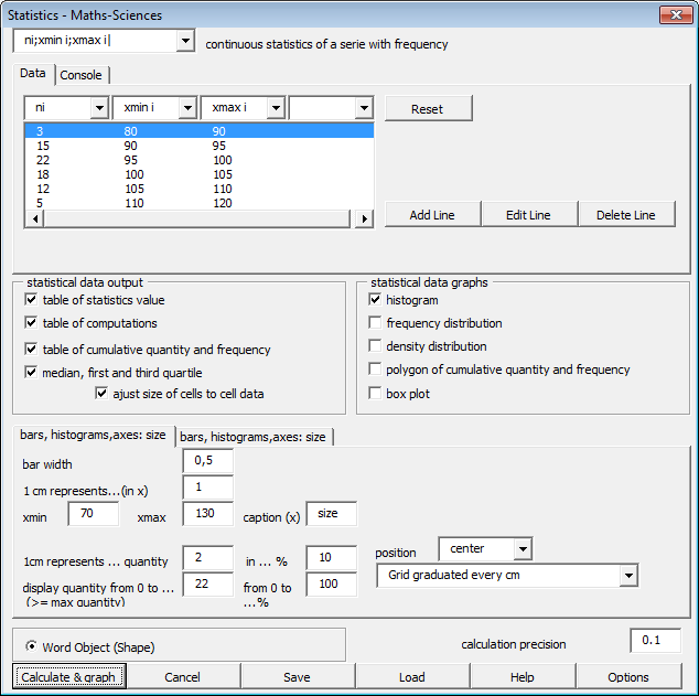
We can get the table of statistics (and table of computations), the quantity histogram, the frequency histogram, the density histogram, and the box plot.
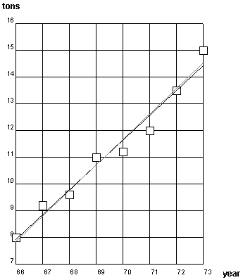
Statistics 7: xi,yi
Linear regression of a data set
Enter the data in a Word table: (here tons of mail delivered)
Then click on the Statistics button:
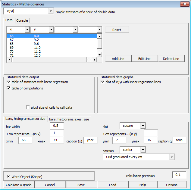
We get the table of the statistics in x, in y and in xy.
We get the regression line with x as variable (first curve color), and with y as variable (second curve color).
We get the table used for calculation.
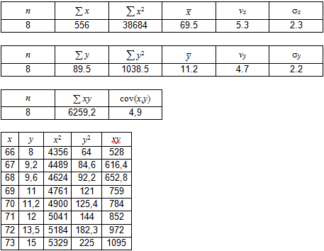
Linear regression in x: y=0.9*x-53.3
Linear regression in y: x=1*y+57.8
Statistics 8: ni,xi,yi
Linear regression of a data set of points with weight
Enter the data in a Word table: (Here number of flats, number of rooms, surface)
Then click on the Statistics button:
We get the table of statistics in x, in y, and in xy.
We get the linear regression with x as variable (first curve color), and with y as variable (second curve color).
We get the table used for calculation.
We get the plot of points - the surface of the plot being proportionnal to the weight of the point, with the regression lines in x and in y.
Linear regression in x: y=16.6*x+15.8
Linear regression in y: x=0.060*y+0.8
Options : see.
Check cell to move each cell of the grid.
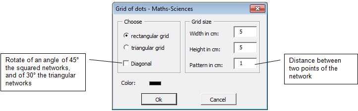
Click on the Graphpaper button displays the dialog box:
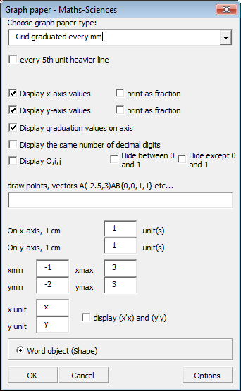
Choose the type of graphpaper
- every millimeter
- every two millimeter
- every centimeter
- every centimeter with half centimeter
- axis graduated every centimeter
- axis graduated every millimeter
- semi-log
- log-log
- polar
Enter the graphpaper intervals.
Enter the name of the axes.
Check the different options: (O,i,j), hide 0 and 1...
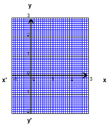
Example : graph paper graduated every millimeter [-1,3]x[-2,3]:
Options: line width and colors.
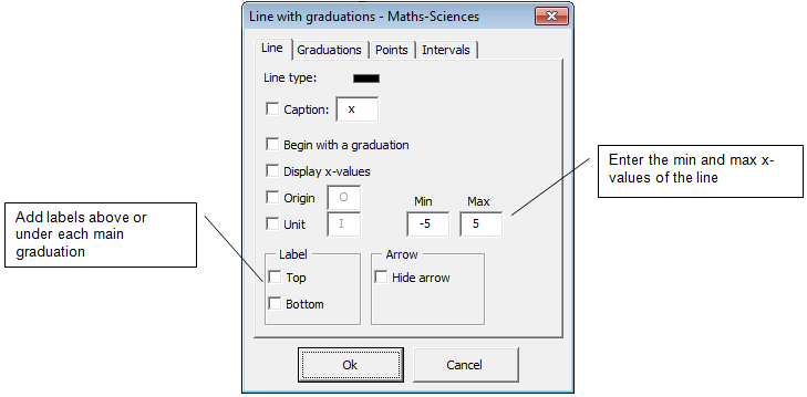
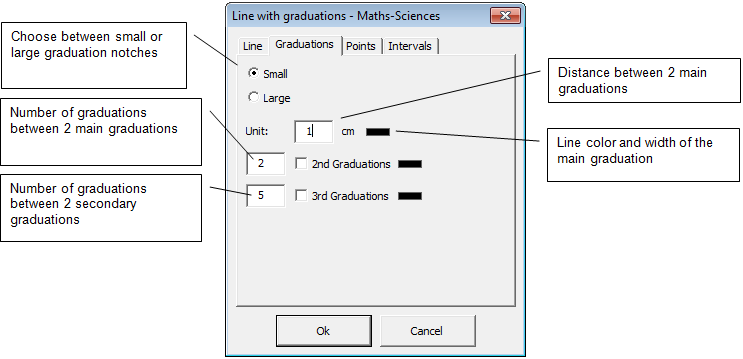
Click on the axis button displays the dialog box:
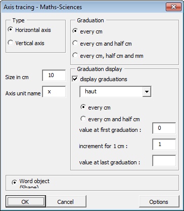
Choose horizontal or vertical.
Enter the axis length.
Choose the type of graduation: every centimeter, every half-centimeter, every millimeter.
Check Display graduations if you want graduations to be displayed.
Enter the start value and the increment between two values.
Example: horizontal axis, 10 cm, graduated every half-centimeter, display graduations start 0 increment 1, unit x :
Options: lines width and color, graduation font.
Click on the Trigonometric circle button displays the dialog box:
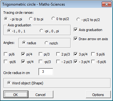
Choose the interval where the circle will be drawn:
- from - p to p - from 0 to p
- from 0 to p/2 - from -p/2 to p/2
Check the options: axis with or without arrows.
Choose between notch and radius.
Enter the radius of the circle.
Example: from - p to p, axes -1, 0 , 1 with arrow, radius 3 cm, angles p/4 3p/4 -p/4 -3p/4:
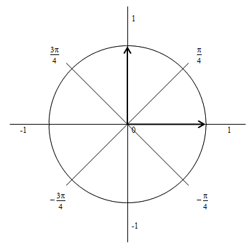
Options: line width and color, font.
Click on the Semi-log and log-log button displays the dialog box:
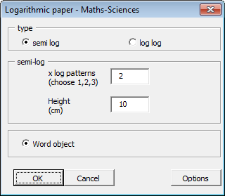
Choose the type of graph paper: semi-log or log-log.
For semi-log, enter
- the number of horizontal logarithmic pattern
- the height in cm
For log-log, enter
- the number of horizontal and vertical logarithmic pattern
Example: semi-log 2 patterns, 10 cm
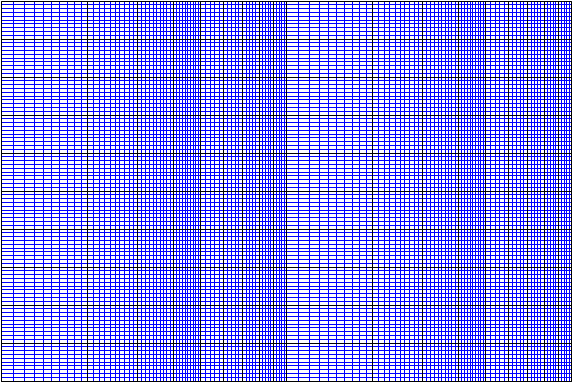
Options: line width and color, size of the logarithmic pattern.
 The Geometre
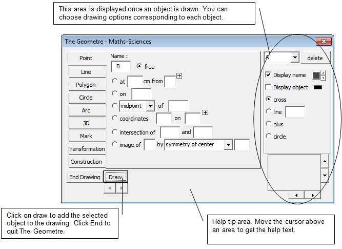
In the Construction tab:
- Scale: the drawing is done at scale 1:1. When The Geometre is closed, the scale is applied.
- Grid:
- magnetism: points will follow the grid.
- hide/display during the drawing. The grid is removed when The Geometre is closed.
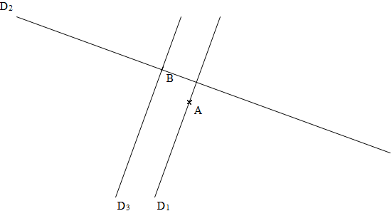
Example for building a geometrical figure:
Type the following text in a text area:
Draw point A
Draw line D1 passing by A
Draw line D2 perpendicular to the line D1
Draw the point B on the line D2
Draw the line D3 parallel to the line D1 passing by B
Then click on run tracing.
The Geometre dialog box opens and asks to place the point A, to orient D1 around A, to place D2 perpendicular to D1, to place B on D2, and draws D3 parallel to D1 passing by B.
The result is:
Ctrl+Shift+M Programmatic Quick Insertions
Drawing:
pen insert a pen
setsquare insert a set square
semicircularprotrator insert a semicircularprotractor
protractor insert a protractor
Geometrical objects (2D):
cross insert a cross with its name
point insert a point with its name
segment insert a segment with 2 text frame for its end-points
equilateral insert an equilateral triangle
isocel insert an isocel triangle
rhombus insert a rhombus
parallelogram insert a parallelogram
rectangle inser a rectangle
Lines:
equil
hexa
line
smallsquare
Geometrical objects (3D):
cuboid
pyramid
cube

sphere
tetrahedron
foldingcuboid
Operators:
arrow insert an arrow
* insert ´
: insert ¸
delta insert the greek letter d
digit- insert the minus sign (calculator font)
digit1 inser the 1 sign (calculator font)
...
digit9 insert the 9 sign (calculator font)
Comparison:
diff insert ¹
app insert »
equivalent insert Û
thereexist insert $
imply insert Þ
forall insert "
lte insert < (less than equal)
gte insert > (greater than equal)
Pi:
pi insert p
pi/2 ...
pi/3 ...
pi/4 ...
2pi/3 ...
Symbols:
ieo insert Î (is element of)
neo insert Ï (not element of)
union insert È (union)
inter insert Ç (intersection)
sbo insert Ì (subset of)
inf insert ¥ (infinity)
|-> insert the definition arrow (to define a function)
0+ insert 0+ (+ as superscript)
0- insert 0- (- as superscript)
Sets of numbers:
All sets can be typed (N, Z, R, Q, D) using the following formating:
r insert the real numbers
r+ insert the positive real numbers
r+* insert the positive real numbers not equal to zero
Ctrl+Shift+Y Automatic Quick Insertions
* ´
-+ ±
+- ?
<= <
>= >
1/2 display the fraction
1/3 in field codes
1/3 using calibri font
alpha a
and Ù
anp display A(n,p)
appr »
appequal @
beta b
c Z
cnp display C(n,p)
congruent º
delta D
diff ¹
drond 
equi Û
ex ex
forall "
hold ?
gamma g
gte >
i display vector i
ieo Î
imp Þ
inf ¥
inter Ç
j display vector j
k display vector k
lambda l
lte <
mu m
n V
n* V*
nabla Ñ
neo Ï
nsbo Ë
nullset Æ
nullv vector null
omega w
or Ú
perp ^
phi j
pi p
pi/2, pi/3, pi/4, pi/6
q X
r Y
r-, r+, r-*, r+*
rond o
sbo Ì
sete display a star
setm display a minus
setme display a minus and a star
setp display a plus
setpe display a plus and a star
sqrx square root of x
thereexist $
theta q
u vector u
union È
v vector v
x2 x square
x3 x cube
z W
zbar z complex conjugate
The Functions tab
Draw function curves with points, segments, lines, vectors and clouds points:
In each tab you can add new objects to the grid such as points, segments, vectors, lines, function curves, conics, clouds of points.
Example.
Compute the expression of a function from given points:
Example.
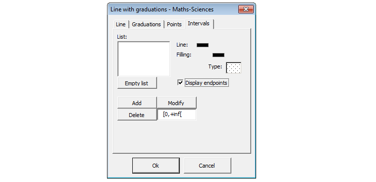
Draw function curves with definition intervals and hashing areas:
Draw curves with scales, graduate axis with scientific numbers, definition intervals, hashing areas.
Example.
Plot points on a grid and link them with segments, arc of paraboles, s-plines:
Plot points on a grid, linking them with segments, arc of parabolas, b-splines.
Example.
Table of values (create or fill existing one) with fractional output :
Case 1: the cursor is on a blank line, a dialog box is displayed to enter the function expressions, and start and end x-values, and the number of values, to compute the expressions.
Case 2: the cursor is in a table cell, however the function expressions are in the first line or in the first column, the table will be filled with the computation of the expressions.
Example.
Variation table of a function defined by its expression:
Enter the function expression, the start and end values, and its turning points ; ex: -inf;-1;0;1;+inf.
Option: display the sign of the derivative.
Exemple.
Variation table defined by the variation it-self:
Example.
Sign table of one or many expressions:
Enter the expressions separated by a comma, start and end x-values, and the values where the sign changes.
Example.
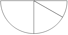
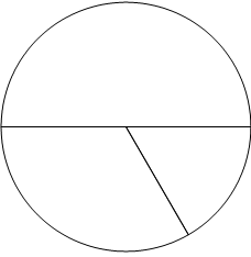
Compute static tables and values of series and draw bar-graphs, pie-diagrams, and box-plots:
Example.
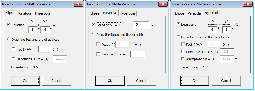
Conics, drawn on a grid:
Example.
Note : Shape = on the page, Canvas = attached to the current line.
The Physics tab
The Equation Editor group:
EQ Not selected: grey : formatting expressions are done with Word Equation Editor.
Selected: yellow or blue: formatting expressions are done with the font defined in the Options and using fields codes.
{a} Display/Hide fields codes.
The Tools group:
Inserts the selected drawing/text in your library of drawing, organize it, and recall them into your documents.
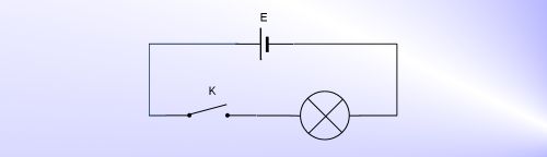
The Electricity group:
Example.
Electricity drawing library.
The Mechanics group:
Mechanics drawing library.
The Optics group:
Example.
Example.
Optics drawing library.
The Acoustics group:
Acoustics drawing library.
The other groups can be displayed with the Group/Tab button in the Scidot tab.

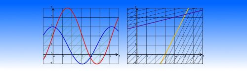
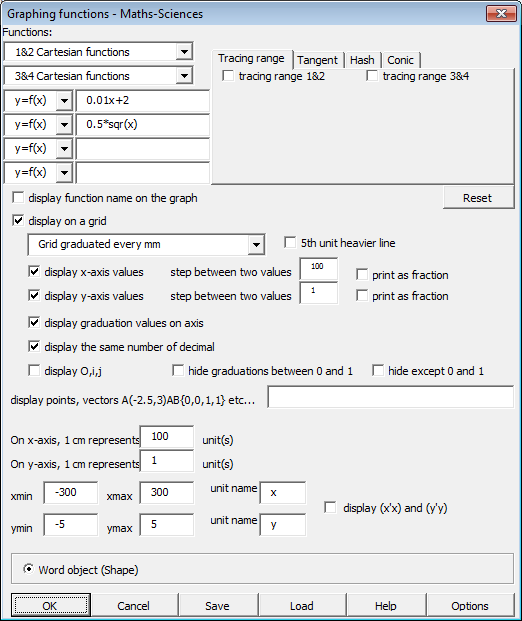
This function grapher can draw one or more functions (on a grid).
To enter the functions:
select the functions expressions separated by commas then click on Graphing Function
or
click on Graphing Function and enter the expressions in the dialog box
Example :
Note: read the Math Expression rules.
A dialog box opens:
Click on Tracing Range tab, then click on the tracing range checkbox to display the textbox to enter the tracing range (one or two intervals).
Click on the Tangent tab to enter the points where a tangent to the function curve will be drawn.
Example: x=1 name of the point:A right and left tangent ; to enter more than one point, enter x=-1 ; 2 then name of the point that will be displayed: A ; B
Click on the Hash tab to define an area the of plane to hash and to choose hash type:
Area of the plane:
y>f(x) or x>g(y) (according to function definition y=f(x) or x=g(y))
y<f(x) or x<g(y) (idem)
surface of the integral sum : 0<y<f(x) (f(x)>0) and f(x)<y<0 (f(x)<0) (respectively for x=g(y))
f(x)<y<g(x) then enter f(x);g(x) in the function definition textbox.
Hash type:
polygone (you can change background color and etc...).
lines: set of lines parrallels to the defined line:
default line is y=x and the space between two line is 0.5
Check Display on a grid.
If left unchecked, the functions will be graphed without gridlines.
Grid type:
a centimeter grid, a half-centimeter grid, a millimeter grid, a two millimeter grid, axes graduated in centimeters, axes graduated in millimeters.
Choose if you want the fifth unit line to be heavier (like on a graph paper)
Check the box if you want to display the x-values and the y-values.
Then choose if you want to display the x-values and the y-values on the bottom and left side, respectively, or along the axes.
Again choose the step of x-values and y-values between two consecutive graduations (by default every centimeter).
If this value is not a multiple of the scale, then a line of axis-width will be drawn for every value.
Display O,i,j and suppress graduations between 0 and 1, suppress graduations except 0 and 1
Enter x-scale and y-scale:
1 cm represents 1 unit : from -4 to 4, the interval length will be 8 cm on the drawing
1 cm represents 2 units : from -4 to 4, the interval length will be 4 cm on the drawing
1 cm represents 0.5 units : from -4 to 4, the interval length will be 16 cm on the drawing
Graphing range
Enter xmin and xmax
Enter ymin and ymax
You can use expressions in the xmin, xmax, ymin, ymax values such as pi/2 , 2/3, etc..
The function curves can go outside these intervals, but only the range will be traced.
The x or y range is rounded to the nearest 1/10th of the scale value :
Ex: from -4.25 to 3.14 with 1cm representing 1 unit will be considered as from -4.3 to 3.1
Increment: dynamic.
Options:
Display min and max range value on grid.
Display graduations as fractions.
Display unit name on x-axis and y-axis:
Example: U[AB] displays U with AB in subscript
Example: f{2} displays f with 2 in superscript
In Word equation editor mode (EQ button is grey), the graduations are displayed using Word equation editor in the size specified (font is Calibria Math).
In Field code mode (EQ button is blue or yellow), the graduations are displayed directly in the font and size specified (field codes are used for fractions).
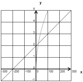
In the following example we have:
A centimeter grid with every fifth line heavier.
x-values and y-values displayed on the axes.
x range : between -3 and 3.4 x scale: 1 cm represents 1 unit
y range : between -1.3 and 5 y scale: 1 cm represents 1 unit
Display : x unit name(x) and y unit name (y) + display opposite unit names
Result:
Example: when the x graduation is not a multiple of the x-scale:
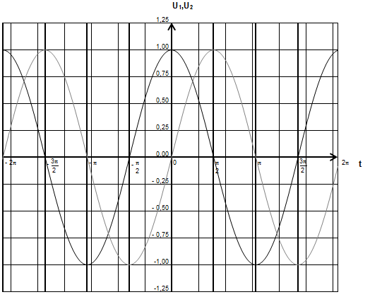
Graphing sin(x) and cos(x) from -2p to 2p with x-graduation every pi/2:
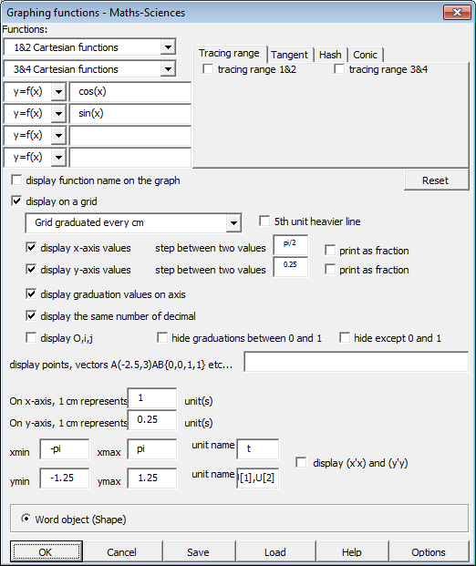
Note: checkbox Display same number of decimal is checked so that instead having 1 , 1.25 , 1.5 we have 1.00 , 1.25 , 1.50...
Note: the checkbox Fraction displays x-axis graduations as fraction (of pi here)
Result :
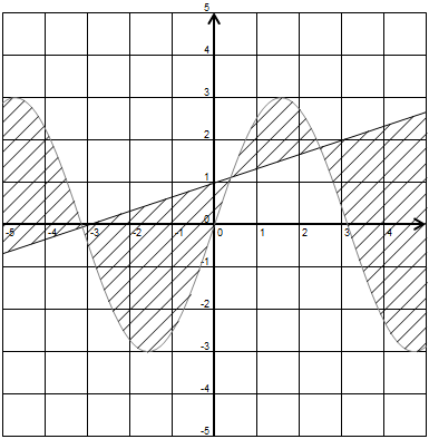
Example with hashed area between two function cruves:
Graph 1+x²/2 and 3*sin(x) defined on -2 , 2 on a grid graduated every cm from -3 to 3 with hashed area of f(x)<y<g(x) :
Result :
When typing x+0.25 pas 0.5, the hashing lines are from the family of lines x+0.25+k*0.5.
Note: in Options : change grid line size and color, axis graduation font name and size, whether to draw the axis x=0 et y=0 with 1/2 cm supplementary on each side, and so on... The changes are saved and kept when you quit Word.
The plotter can draw from one to three sets of points:
- x1, y1, y2 for one x-value, one or two y-value
- x', y'1 for one x-value, one y-value
For each set of points (x,y), you can choose to draw :
- the points
- link the points with lines
- draw a parabolic smoothering
- draw the Bezier smoothering curve (based on middle points)
- draw the spline (N order) smoothering curve
- draw the linear regression line y=ax+b (not x=cy+d)
Prepare the data in a Word table:
The first row contains the set x
The second row contains the set y1
The third row contains the set y2
The fourst row contains the set x'
The fifth row contains the set y'1.
Note: if the first column of the first row contains 'x' then this column will be deleted from the data.
Example: pH measured while titrating 10 ml of acetic acid 0.1M and while titrating 10 ml of ammonia 0.1 M
Place the cursor in the table, then click on the Plotter button.
(each set of points can have different number of points)
A dialog box is displayed:
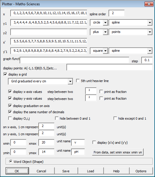
The sets of points are displayed in the dialog box separated by commas.
Facing x, we find the data of volume of strong base used for titration while titrating the acetic acid
Facing y1, we find the measure pH, the choice for the plot (plus, circle, cross, square), and the kind of curve to display
Facing y2, we find ,,,,,,,,,,,,,, (empty line in the table) that shall be deleted.
Facing x', we find the data of volume of strong acid used for titration while titrating ammonia
Facing y1',we find the measure pH, etc...
This dialog box is quite similar to the function graphing dialog box.
In the example, the domain of the x-interval is from [xmin=0 , xmax=20] with an x-scale of 1 cm representing 2 units
and the range of the y-interval is from [ymin=0 , ymax=14] with a y-scale of 1 cm representing 1 unit.
More over you can graph functions and draw points A(x,y) and vectors AB(0,0,1,1)
- add one or more functions f(x);g(x);... that will be drawn
- add a set of points and vectors
Result:
The titration measurement gives the following picture:
Note: read the options.
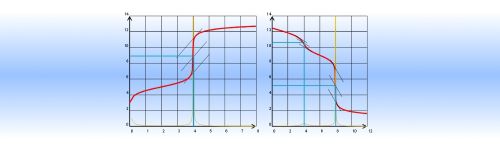
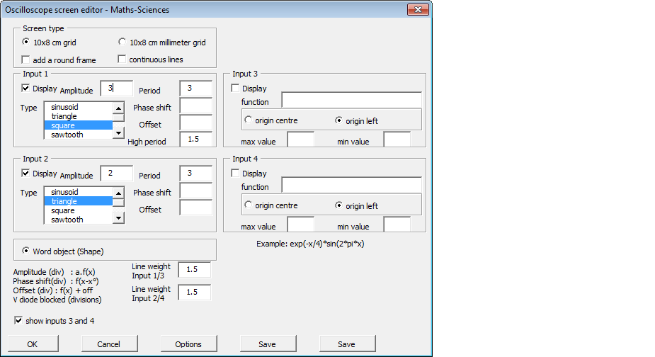
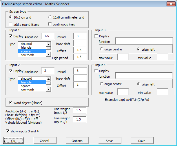
The oscilloscope screen editor can draw from one to four curves.
Click on the Oscilloscope Screen Editor button to display the following dialog box:
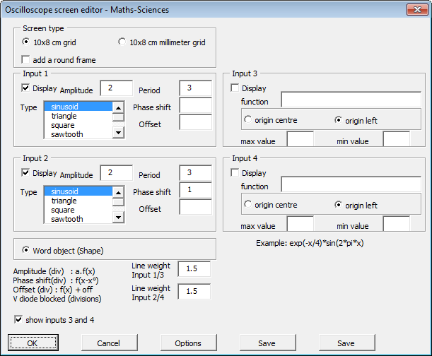
Chose the oscilloscope screen (10cm x 8 cm) type:
- grid every centimeter or every millimeter
- with or without a rounded frame
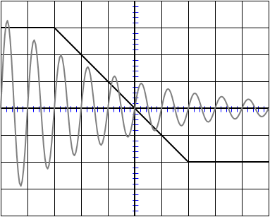
When drawing one or many square curves, choose if you want the curves to be continuous or not.
For the oscilloscope input 1 and 2:
Click on display to include the input in the finished drawing.
Choose the input type:
sinusoidal/triangular/square/diode/backward diode/rectification/inverse rectification/load-unload
Enter the amplitude and the period as measured in screen squares (1 cm).
Enter the phase shift measured in screen squares. A positive phase shift indicates the input is in advance.
Optionaly, enter the offset value measured in screen squares (a constant added to the input).
For a square input, enter the time value where the value is on the upper value.
For a diode, enter the value of the tension when the diode is blocked (for zener).
For a capacitor load/unload, enter the inverse of the RC delay measured in screen squares.
For the oscilloscope input 3 and 4:
Click on display to include the input in the finished drawing.
Enter the the oscilloscope curve function expression
The function is graphed on a 10 unit x 8 unit grid.
Choose between the origin on the center (0;0) or on the left (-5,0)
Enter the maximum value if required. Enter the minimum value if required.
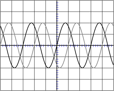
For example:
Input 1 : Sinusoidal : amplitude 2 : period 3
Input 2 : Sinusoidal : amplitude 2 : period 3 : phase shift 1
Result:
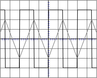
Example 2 : square signal integration
Input 1 : square : amplitude 3 : period 3 : high period 1.5 (low period = period (3) - high period (1.5) = 1.5)
Input 2 : triangle : amplitude 2 : period 3
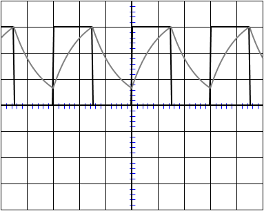
Example 3 : capacitor load-unload
Input 1 : square : amplitude 1.5 : period 3 : offset 1.5
Input 2 : load/unload : amplitude 3 : period 3 : inverse of delay 1
Example 4 : use of function to graph oscilloscope inputs
Input 1 : function - x : origin on the center of the grid
Input 2 : exponential damping function : exp(-x/4)*sin(2*pi*x)
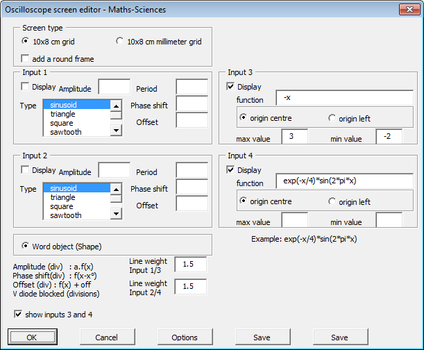
Note: Click on options to access the color options (identical to the Function Graphing and Plotter options).
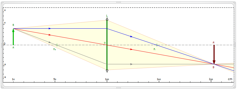
With the optical bank you can draw rays through one or two converging or diverging lens.
You can also display usual optical instruments.
Rays are drawn using the geometric optic laws.
Optical bank:
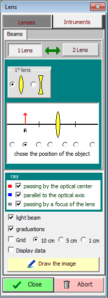
Choose the type and number of lens and their approximate position.
Click on Construct the Image.
A first drawing is made.
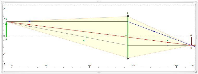
Then click on the Modify tab, enter the precise values of the bank and ask to redraw.
You can draw a grid and display the values of OA, AB, OA', A'B'.
Result:
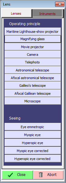
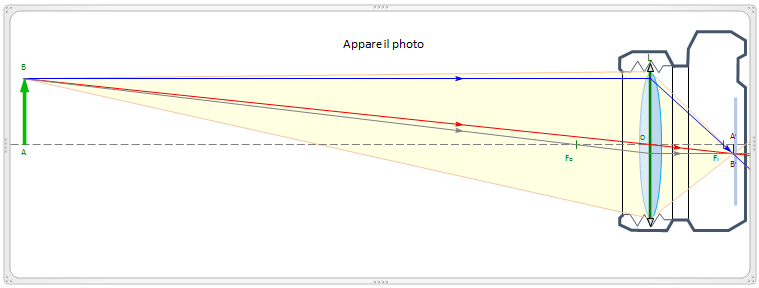
Optical instruments:
Exemple: camera
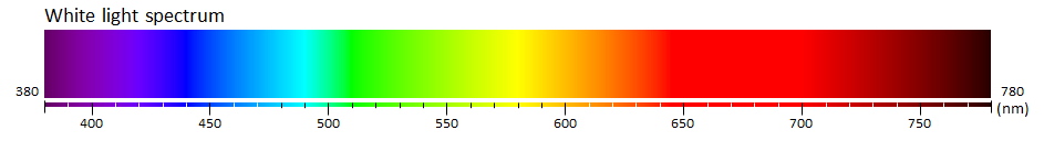
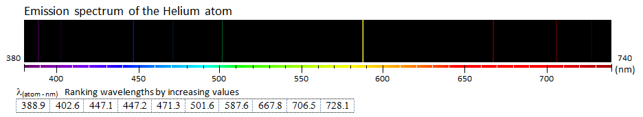
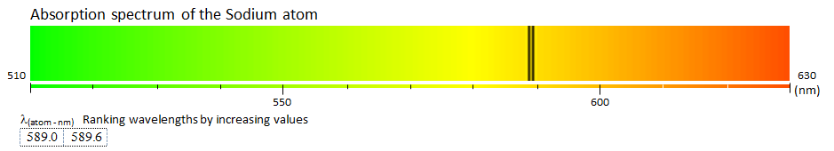
The Spectrum tool inserts White Light Spectrum, and Emission and Absorption Spectrum of all chemical elements.
Click on the Spectrum button opens :
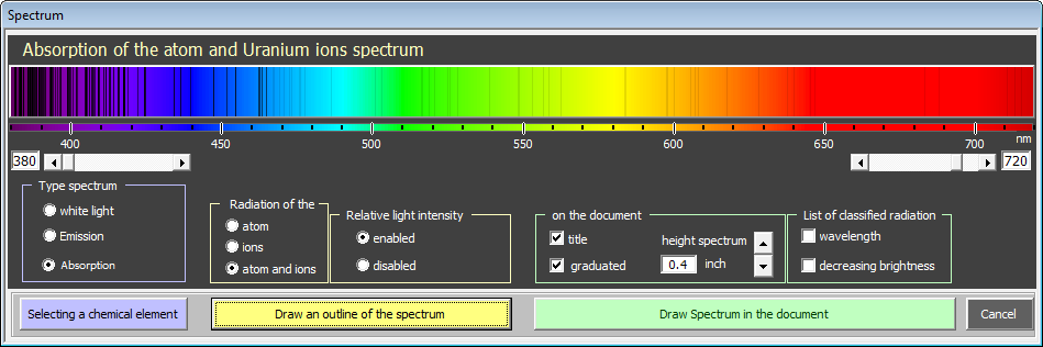
Left and right cursors allow to define low and upper limits of the spectrum.
With type of spectrum, you can choose between while light, emission and absorption.
Radiation allows you to choose between atom, ions, and atom and ions.
Relative light intensity displays a line with a lower brightness according to the intensity of the ray.
On the document : ouput options.
You can ask to print out rays by decreasing wavelength (default) or by decreasing brightness.
White light spectrum:
Helium emission spectrum:
Sodium absorption spectrum:
The Chemistry tab
The Equation Editor group:
EQ Not selected: grey : formatting expressions are done with Word Equation Editor.
Selected: yellow or blue: formatting expressions are done with the font defined in the Options and using fields codes.
{a} Display/Hide fields codes.
The Tools group:
Inserts the selected drawing/text in your library of drawing, organize it, and recall them into your documents.
The Writing group:
The Function group:
Example.
Example.
Example.
Example.
The Chemical arrow group:
The 3D group:
Example.
The 2D group:
Example.
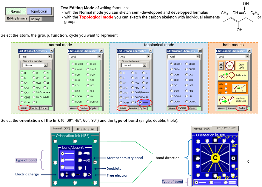
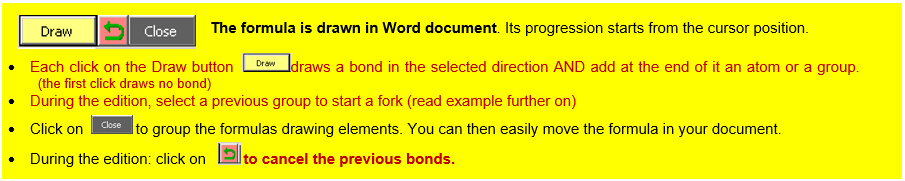
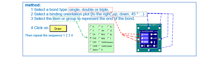
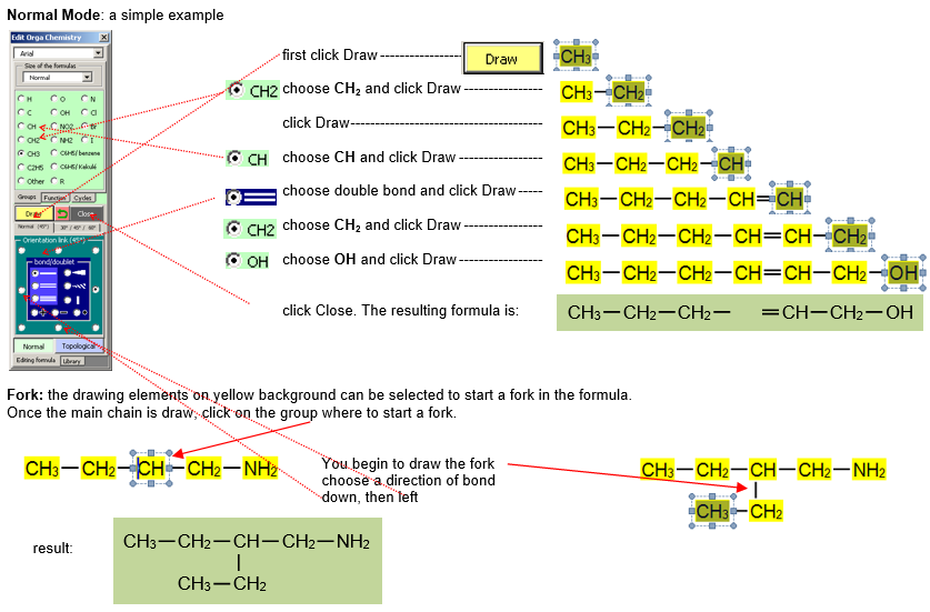
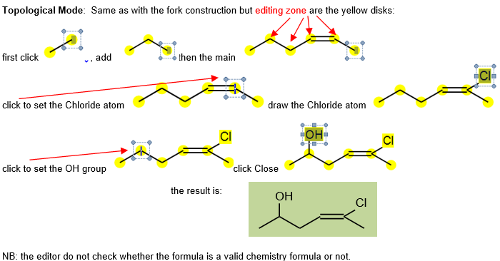
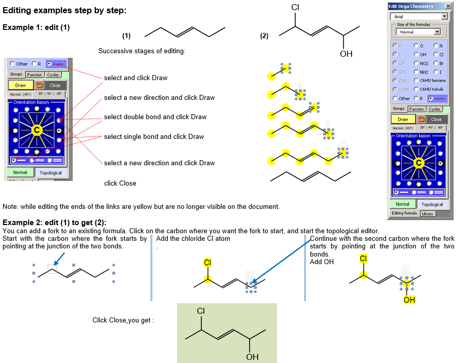
The chemical formula editor:
Editor menu.
Example.
This command format the selection or the text in the dialog box as a chemical formula.
result:
This command compute the molar mass of a chemical formula from the selection of a dialog box.
This command can draw titration curves and table pH=f(v) when titring acid(s) by a strong base.
The computation of the pH is done using dichotomy on the chemical solution equations.
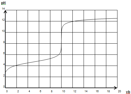
Example: titration of 100 mL of ethanoic acid (pKa = 4.7) of concentration 0.01 M by sodium hydroxide of concentration 0.1 M
Click on the Titration of acids by strong base to display a dialog box:
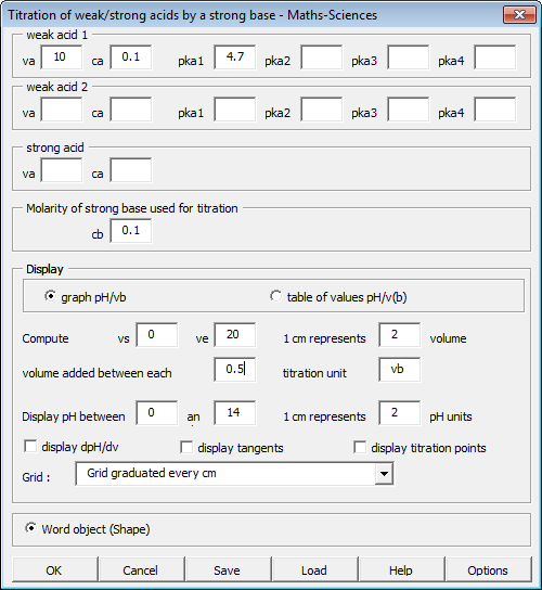
You can enter :
a first weak acid with up to 4 dissociations.
a second weak acid with up to 4 dissociations.
a strong acid
In the example:
V(a) = 100 mL M(a) = 0.01 M pKa = 4.7
No other acid
Concentration of the strong base
M(b) = 0.1M
Graph ph=f(V(b)):
Display pH between 0 and 14 ; 1 cm represents 1 pH unit
Titrate between Vi = 0 mL and Vf = 20 mL (10 mL will be the equivalence volume)
Grid : centimeter grid
Result:
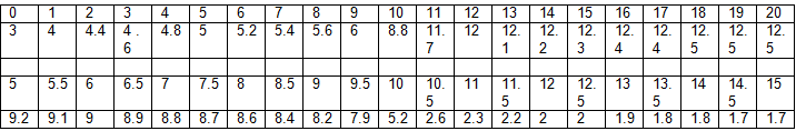
A table of values between Vi = 0 mL and Vf = 20 mL, increment 1 mL :
Example 2: titration of 50 mL of sulfuric acid (first dissociation is strong, second is weak pKa = 2.1) of concentration 0.08 M by sodium hydroxide of concentration 0.1 M
Equivalent volume expected Vb = 40 mL for the first strong acidity,
Vb = 80 mL for the second weak acidity
Enter the sulfuric acid as a mixture of
a strong acid of 50 mL of concentration 0.08
a weak acid of 50 mL of pKa1 = 2.1 of concentration 0.08
(the equivalence can be found in the chemical equations)
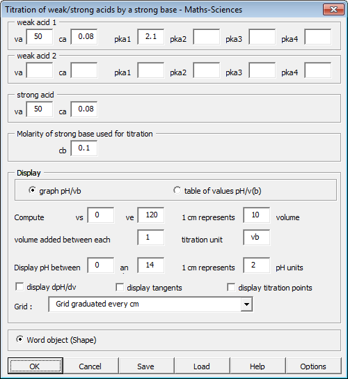
Result:

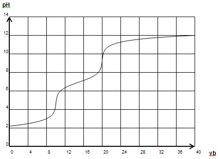
Example 3: titration of 100 mL of orthophosphoric acid (three weak dissociations pKa = 2.1 ; 7 ; 12.1) of concentration 0.01 M by sodium hydroxide of concentration 0.1 M
Equivalent volumes expected vb = 10 mL (first amphoteric)
vb = 20 mL (second amphoteric)
vb = 30 mL (weak base)
Titrated between vi = 0 mL and vf = 40 mL
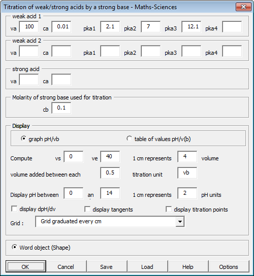
Result:
This command can draw titration curves and table pH=f(v) when titring acid(s) by a strong base.
The computation of the pH is done using dichotomy on the chemical solution equations.
Example: titration of 100 mL of ammonia (pKb = 14 - pKa = 14 - 9.2 = 4.8) of concentration 0.01 M by chlorhydric acid of concentration 0.1 M
Click on the Titration of bases by strong acid to display the following dialog box:
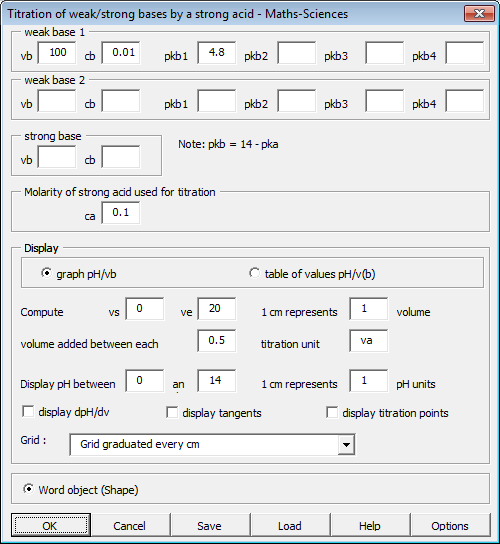
In the example:
V(b) = 100 mL M(b) = 0.01 M pKb = 4.8 (The pKb value = 14 - pKa)
No other weak bases added
Concentration of the acid used for titration
M(a) = 0.1 M
Display the pH between 0 and 14, 1 cm represents 1 pH unit
Titrate between Vi = 0 mL and Vf = 20 mL (10 mL will be the equivalent volume)
Centimeter grid.
Result:
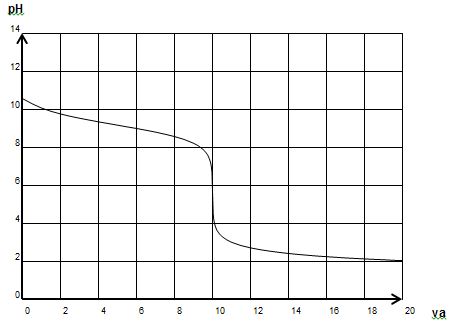
A table of values between Vi = 0 mL and Vf = 20 mL increment 1 mL:
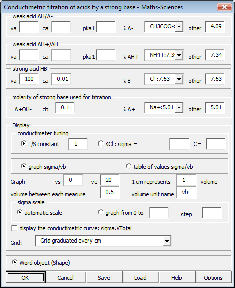
This command can draw conductimetric titration curves and titration tables of values.
The first curve s is computed with the dilution, but you can also draw s.Vt. You can then keep either or both s and s.Vt.
Example: conductimetric titration of 10 mL of ethanoic acid (pKa = 4.7) of concentration 0.1 M by sodium hydroxide of concentration 0.1 M
Click on the Conductimetric Titration of acids by strong base to display a dialog box:
You can enter :
a first weak acid
a second weak acid
a strong acid
In the example:
V(a) = 10 mL M(a) = 0.1 M pKa = 4.7
No other acid
Concentration of the strong base
M(b) = 0.1M
Graph s and s.Vt (volume)
Display pH between 0 and smax
Titrate between Vi = 0 mL and Vf = 20 mL (10 mL will be the equivalence volume)
Grid : centimeter grid
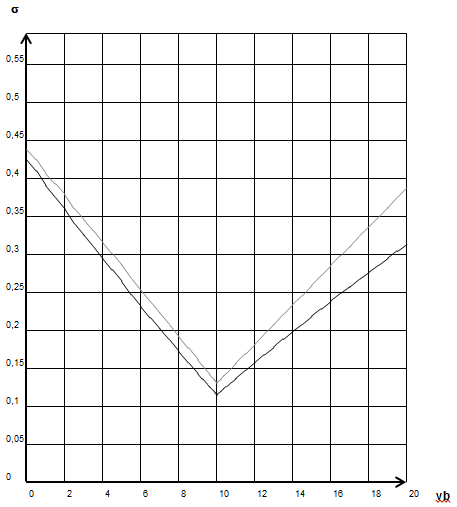
Result:
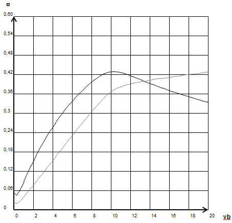
The curve made of lines if the second curve : s.Vt.
Example 2: titration of 50 mL of chlorhydric acid of concentration 0.1 M by sodium hydroxide of concentration 0.1 M
Equivalent volume expected Vb = 10 mL
Result:
This command can draw conductimetric titration curves and titration tables of values.
Example: titration of 10 mL of ammonia (pKb = 14 - pKa = 14 - 9.2 = 4.8) of concentration 0.1 M by chlorhydric acid of concentration 0.1 M
Click on the Conductimetric Titration of bases by strong acid to display the following dialog box:
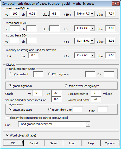
In the example:
V(b) = 100 mL M(b) = 0.01 M pKb = 4.8 (The pKb value = 14 - pKa)
No other weak bases added
Concentration of the acid used for titration
M(a) = 0.1 M
Display G between 0 and Gmax
Titrate between Vi = 0 mL and Vf = 20 mL (10 mL will be the equivalent volume)
Centimeter grid.
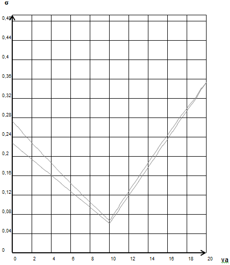
Result:
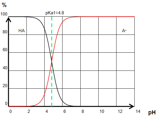
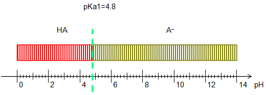
This command can draw the predominance diagram of an acid/base: %(acid/base) according to pH, and also the predominance axis.
Example : predominance diagram of the acetic acid (pKa = 4.8)
Click on the Predominance diagram button to enter the following dialog box:
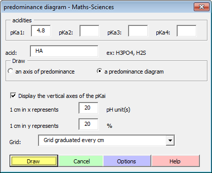
pKa = 4.8 (you can enter up to a quadri-acid)
acid HA : acid names are computed automatically
1 cm = 2 pH units
1 cm = 20 %
Graphpaper : grid graduated every cm (same option as Graphing Functions)
Result for a predominance diagram:
Result for a predominance axis:
Insert a Chemical symbol.
Result:
This command allows you get a table showing the progression of a chemical reaction :
- first line, quantity of reactive
- intermediate line, intermediate state
- last line, quantity of reactive being used in the reaction
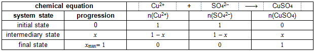
Example: Cu2+ + SO42- = CuSO4
Click on the Progression table button to enter the dialog box:
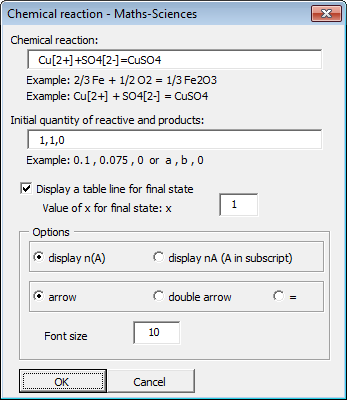
Enter the chemical reaction.
You can choose to display an arrow, a double way arrow, an equal sign.
You can choose to display quantity of reactive between brackets or in subscripts.
Result :
Note: you must compute the xmax value.
Chemical arrows
This group inserts chemical arrows.
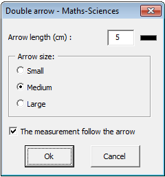
If you want to place text above or under the arrows, select it and click on the arrow button.
When no text is selected, the arrow is inserted without any text.
Options: The arrow length and font size, and the selected text font size.
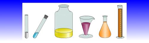
 3D Glassware and apparatus
This command inserts 3D chemistry drawings:
Glassware
- test tube
- beaker
- erlenmeyer flask
- flat bottom balloon (small or wide mouth)
- round bottom balloon (small or wide mouth)
- conic flask
- flask
- measuring flask
- large flask
- measuring cylinder with mouth
- measuring cylinder without mouth
- conic funel
- spheric funel
- burette
- 20mL, 10mL, 5 mL pipette
- volumetric pipette
- syringue
- crystalliser
Apparatus
- magnetic stirrer
- electronic balance
- bunsen burner
- bunsen burner with watch
- calorimeter
- conductimeter
- pH-meter
- matel stand
- pocket pH-meter
- funel stand
Equipment
- reflux heating
- coal combustion (with or without sparks)
- dean-stark
- dilution 1/10
- fractionated distillation
- titration of an acid
- titration of a base
- titration using permanganate
- simple extraction
- simple filtration
- vacuum filtration
- hydrodistillation
- gas reception
Danger symbols
- explosive
- oxidising
- highly flammable
- extremely flammable
- toxic
- very toxi
- iritant
- harmful to health
- corrosive
- dangerous for the environnement
New danger symbols
- cancerigen
- comburant
- corrosive
- ecotoxic
- explosive
- gaz pressure
- inflammable
- irritant
- toxic
This command inserts 2D chemistry drawings:
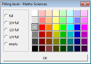
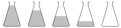
When clicking on a chemistry glassware drawing button, a dialog box is displayed allowing you to select one of five levels of fill: empty, a quarter full, half full, three quarters full, full, and to choose the filling color:
Example (erlenmeyer):
The chemical formula editor form
Three editing actions
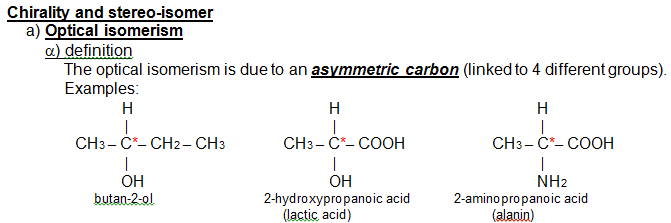
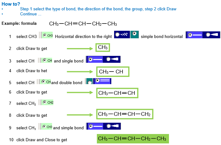
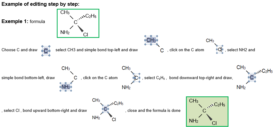
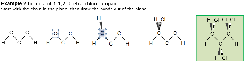
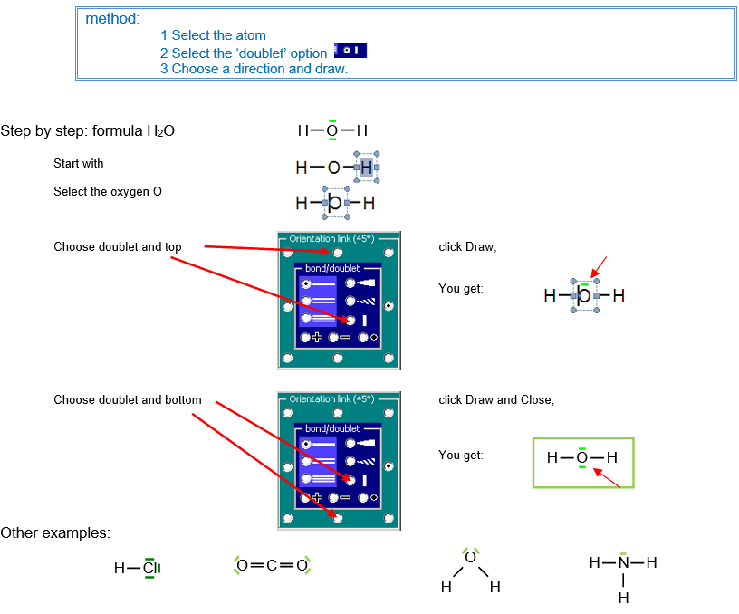
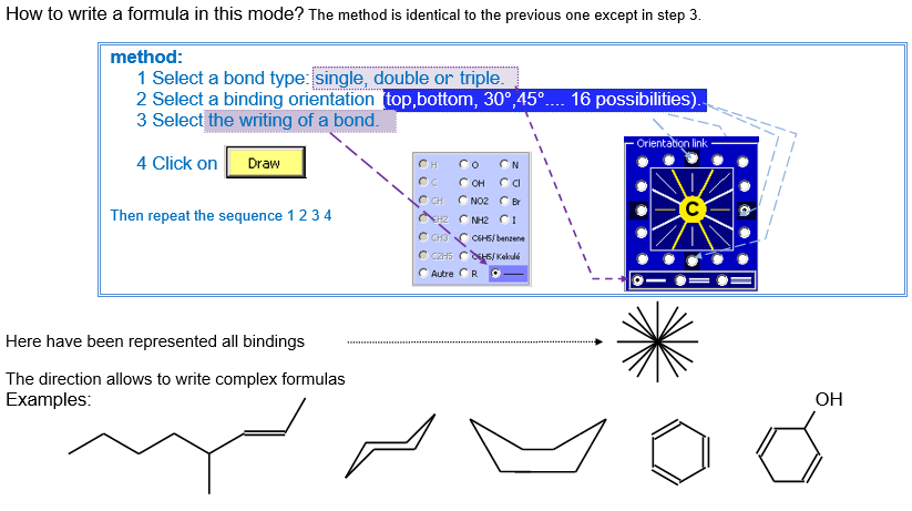
How to write a formula ?
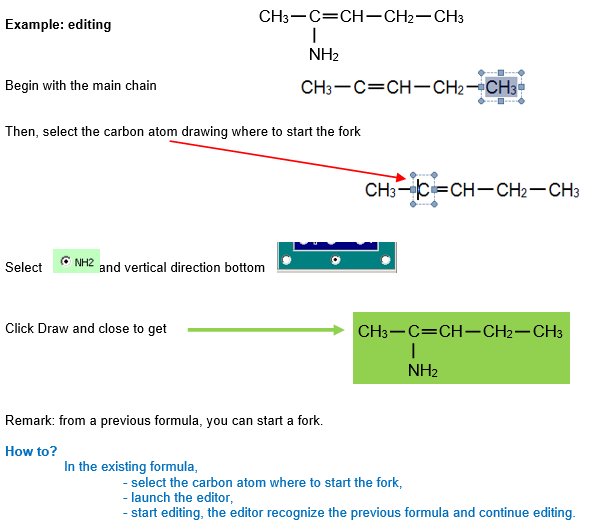
Editing semi-developped formulas without forking
Editing developped formulas with forking
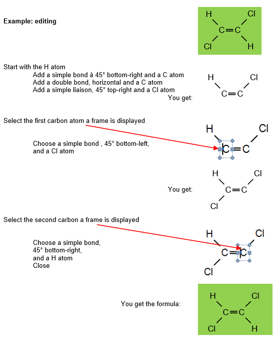
Editing semi-developped formulas with forking
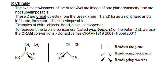
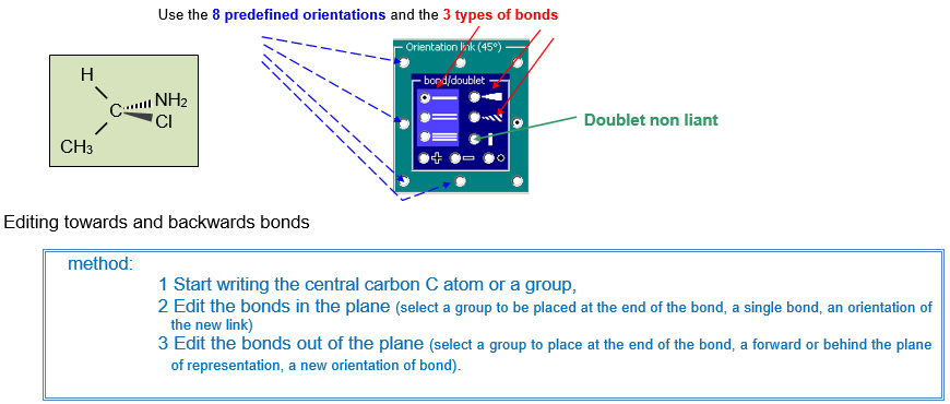
Cram Formulas
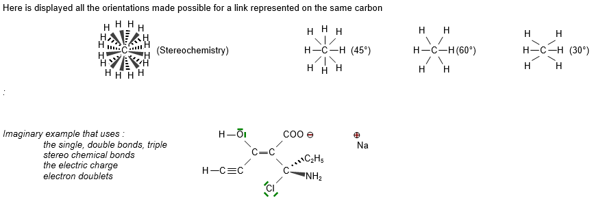
Drawing non binding doublets
Toplogical formulas
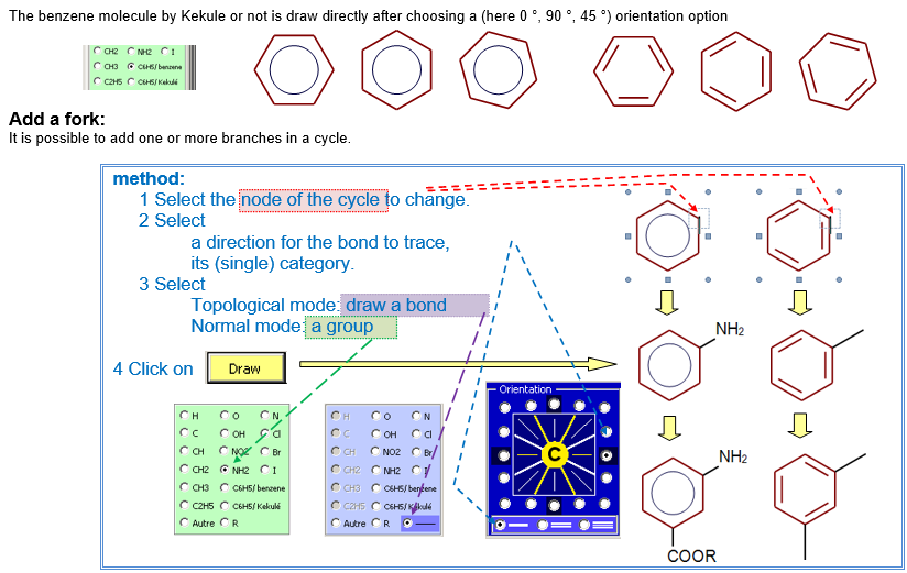
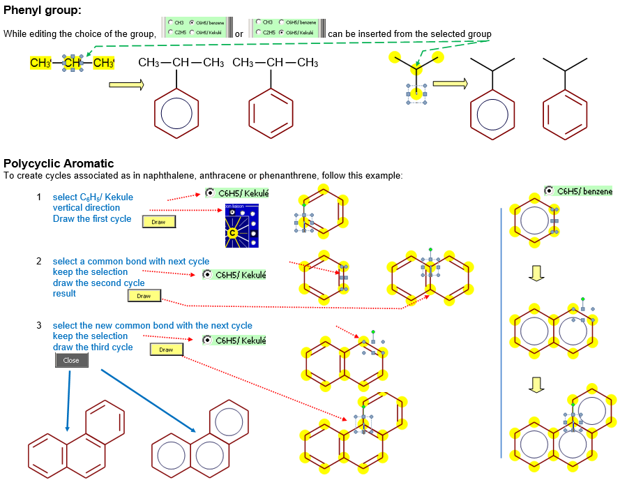
Aromatic molecules
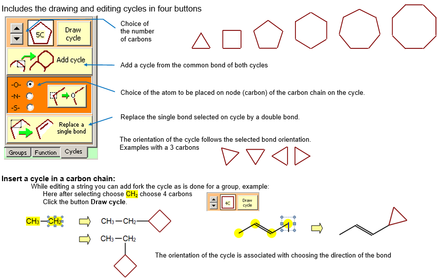
Cycles
Associated cycles
Library of formulas
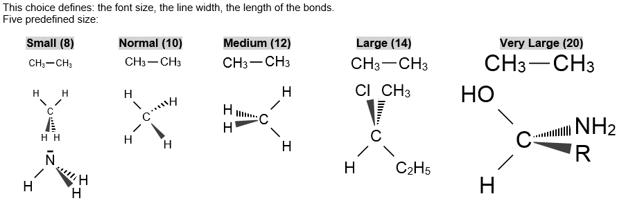
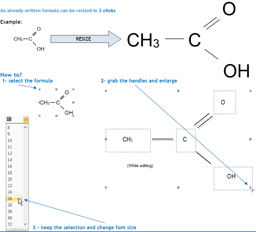
Size of the formulas
The Scidot Tab
The Options and help group:
You will find other options in the dialog boxes.
The Misc group:
The Register group:
The Information group: